WISAN testing on a bridge
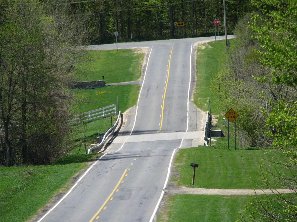
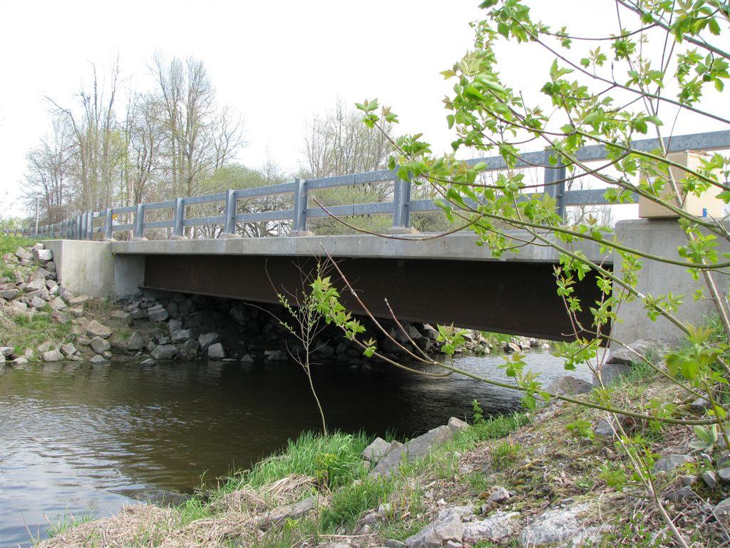
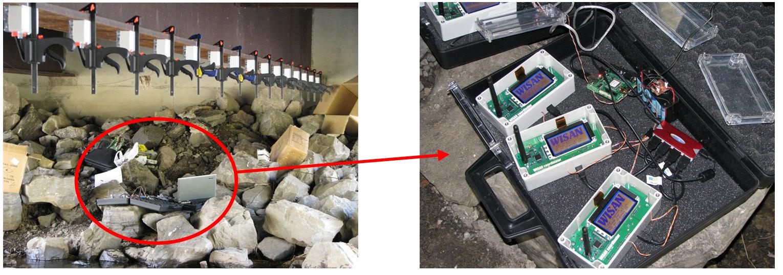
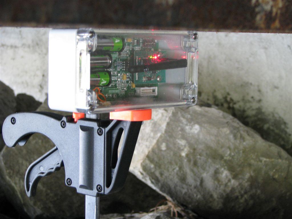
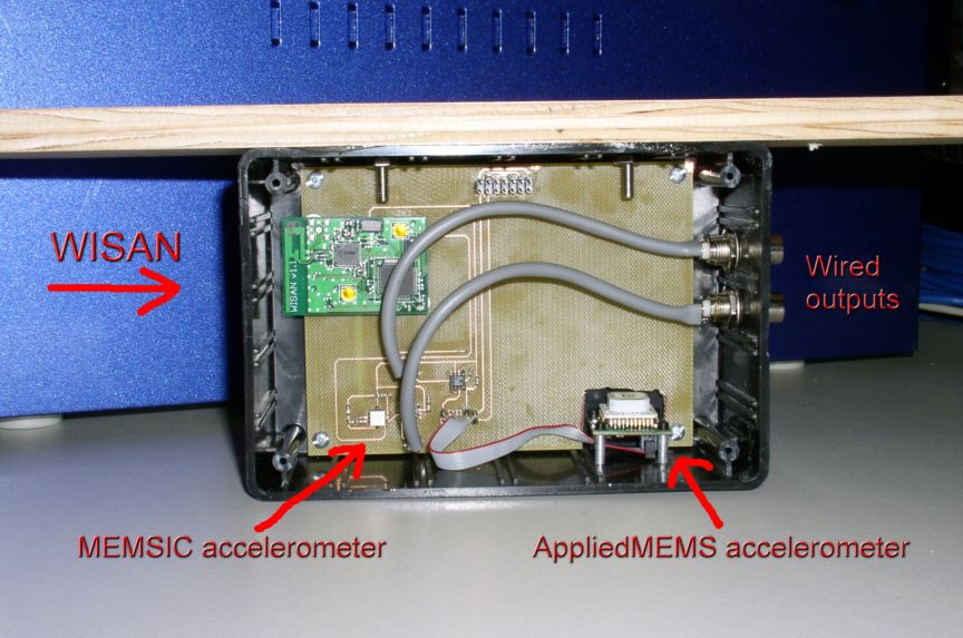
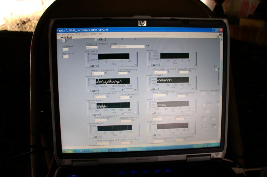
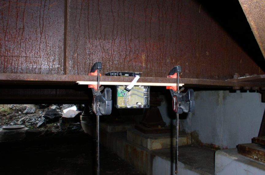
The bridge (Figure 1(a)(b)) was tested in 2 setups using 44 sensors in on two girders and four girders respectively. The sensors were clamped on the bottom of the girders to provide a clear line-of-sight to the PAN Coordinator station (Figure 2) placed under the bridge on the bottom left of the entire setup. The PAN Coordinator station consisted of 6 PAN Coordinators connected to a laptop via serial interface. GPS was used to provide pulse per second synchronization signal to the PAN Coordinators. TCP based server was used to send / receive data from the network. LabView based client application was used to control the data collection process. The network configuration for the tests is shown in Figure 3.
The sensors formed six network clusters on six independent frequency channels that synchronized within ±23 µs using a synchronizing signal provided by the GPS receiver. Acceleration data was sampled at the rate of 240.385 Hz and a data resolution of 14 bits. Traffic passing over the bridge was the source of bridge excitation. Number of data recordings for the three setups were taken for 30 seconds, 2 minutes, 5 minutes and 10 minutes were taken. The cut of frequency of the programmable filter was varied between 100 Hz and 40 Hz to filter out high frequency noise components. Figure 4 shows a time series data for a sensor located near the center of the second girder. The frequency spectrum of the data shows peak amplitude of around 25 mg in the range of 8 – 12 Hz. This corresponds to roughly 6% of the total resolution of the ADC and which is approximately only 6 bits of sensor resolution which is much lower to that seen from the bridge on Route 11 in Potsdam.
(a) (b)
Figure 1: Different views of the bridge on Chipman Road
.jpg)
.jpg)
(a)
(b)
(c)
Figure 2: (a) Placement of WISAN sensors under the bridge (b) PAN Coordinator Station (c) Wireless Sensor clamped to the girder on the bridge
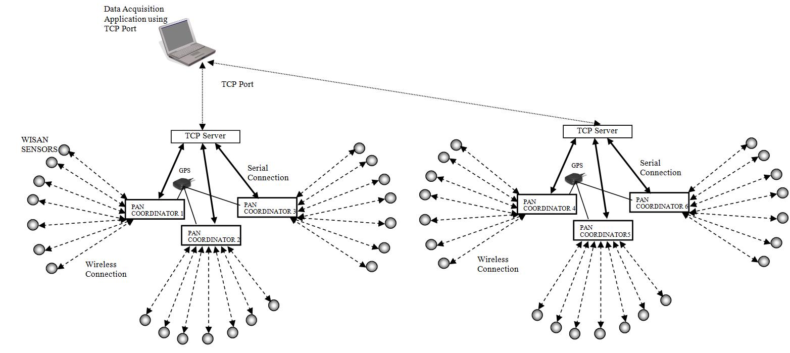
Figure 3: Network configuration for bridge testing (click to enlarge)
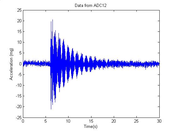
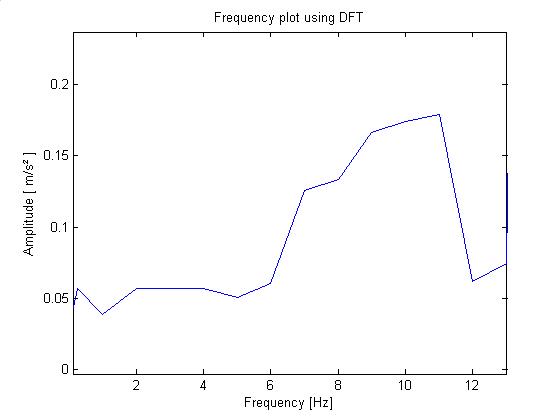
Figure 4: (a) Acceleration data from sensor located near the center of second girder. (b) Frequency spectrum of data from sensor located near the center of second girder.
Four Girder Grid Setup
In the first setup, all four girders were equipped with 11 sensors each. The layout of the test setup is shown in Figure 5.
.jpg)
Figure 5: Layout of the bridge test setup for the four girder grid setup
The data collected from all the sensors was processed using the output-output modal analysis software ARTeMIS. Mode shapes from the four girder grid setup were successfully identified as summarized in Table 1 and shown in Figure 6 – Figure 10.
|
Mode Number |
Frequency (Hz) |
|
1 |
9.155 |
|
2 |
32.75 |
|
3 |
53.65 |
Table 1 (a): Vibration modal frequencies along the length of the bridge
|
Mode Number |
Frequency (Hz) |
|
1 |
10.97 |
|
2 |
26.23 |
Table 1 (b): Vibration modal frequencies along the width of the bridge
.jpg)
.jpg)
Figure 6: Three dimensional view of the first mode at 9.155 Hz obtained along the length of the bridge for four girder grid setup
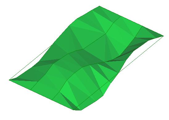
Figure 7: Three dimensional view of the second mode at 32.75 Hz obtained from four girder grid setup
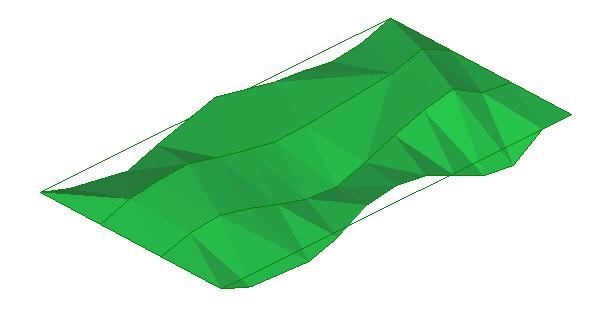
Figure 8: Three dimensional view of the third mode obtained at 53.65 Hz obtained from four girder grid setup
.jpg)
.jpg)
Figure 9: Three dimensional views of the first mode at 10.97 Hz obtained along the width of the bridge (side mode)
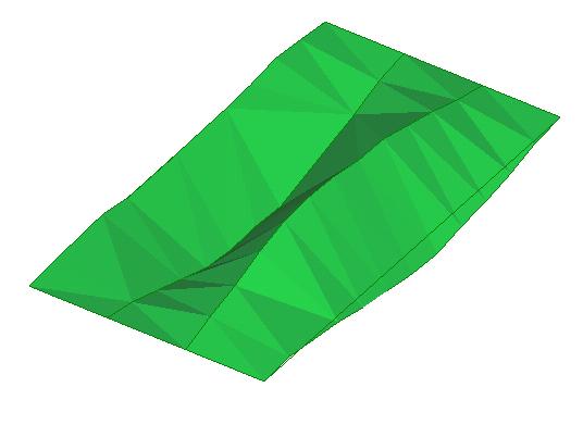
Figure 10: Three dimensional view of the second mode at 26.23 Hz obtained along the width of the bridge
Two girder grid setup
In the second setup, first two girders were equipped with 22 sensors each as shown in Figure 11. The mode shapes obtained are shown in Figure 12 to Figure 15.
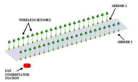
Figure 11: Layout of the bridge test setup for the two girder grid setup
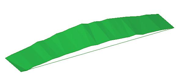
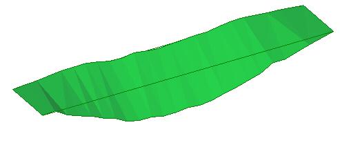
Figure 12: Three dimensional view of the 1st longitudinal modes identified at 9.155 Hz using the two girder grid setup.
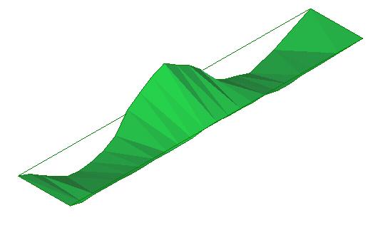
Figure 13: Three dimensional view of the 2nd side modes identified at 26.23 Hz using the two girder grid setup.
 Sensor location close to a support column.
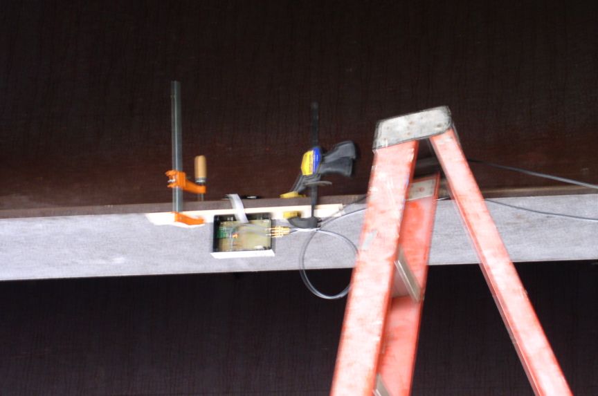 First sensor location. Midspan of the girder
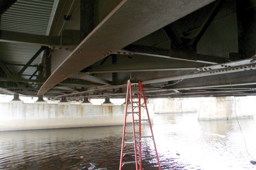 First sensor location. Midspan of the girder.
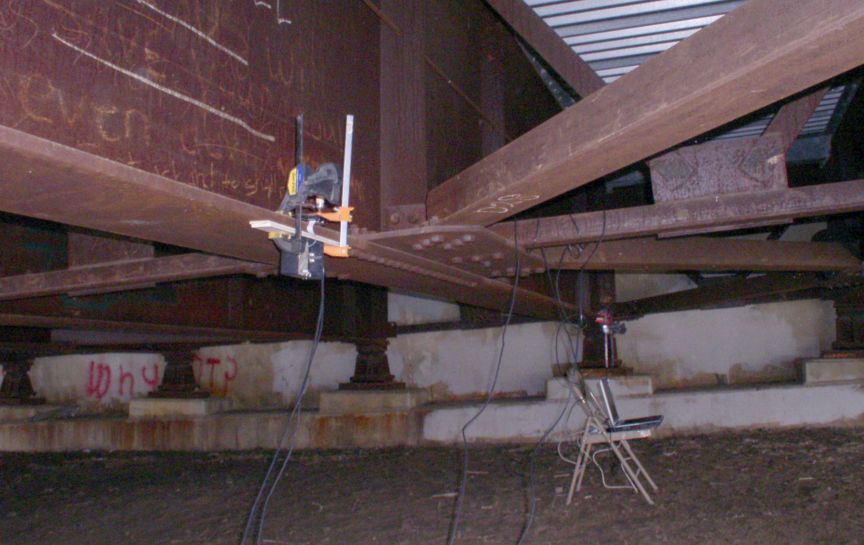 Second sensor location: Moving closer to the support.
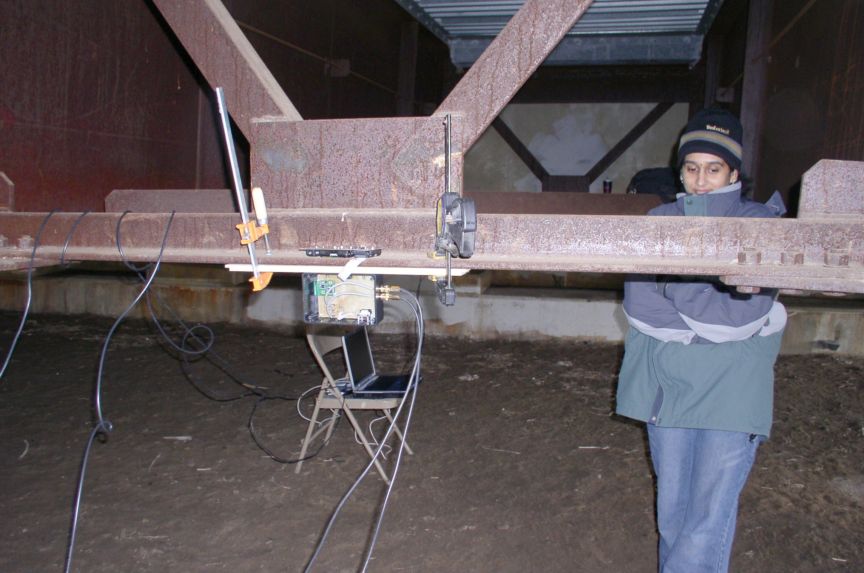 Third sensor location


