May 2008. WISAN experiments on a pre-steressed concete bridge in Kuala Lumpur, Malaysia

Testing of a concrete prestressed bridge

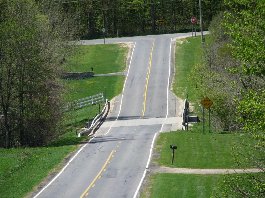
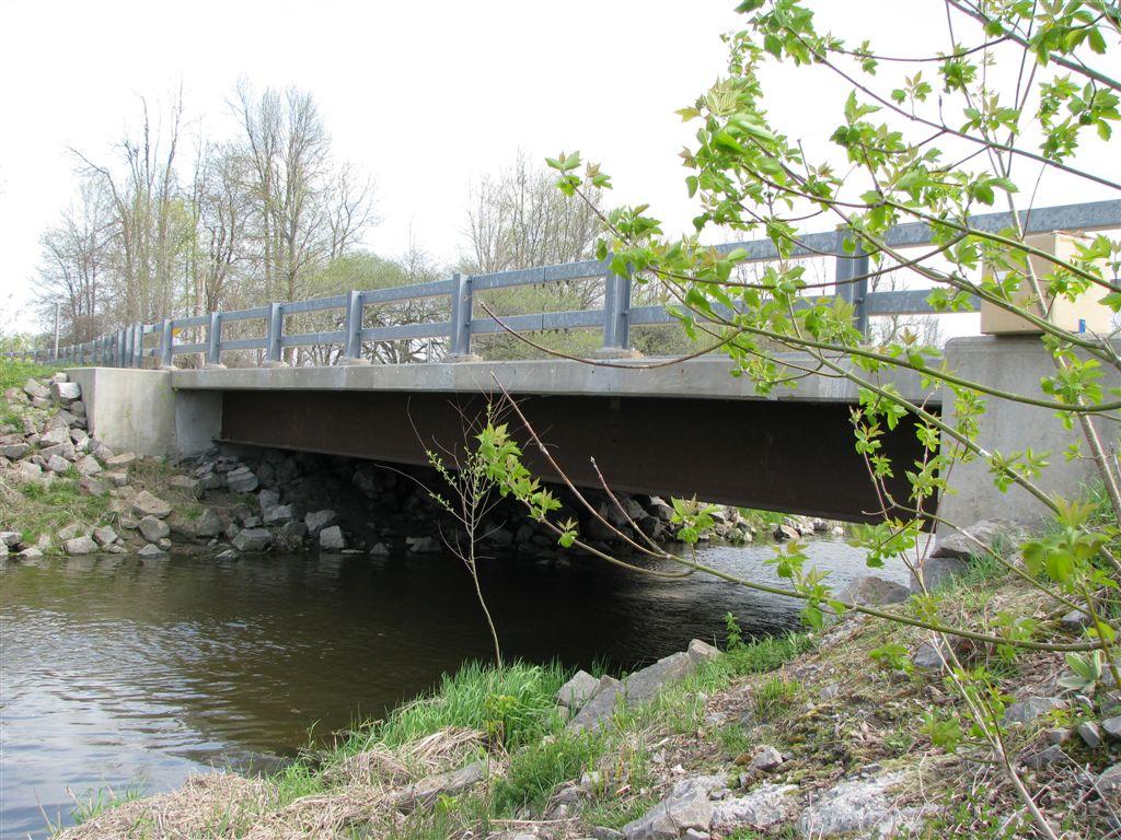
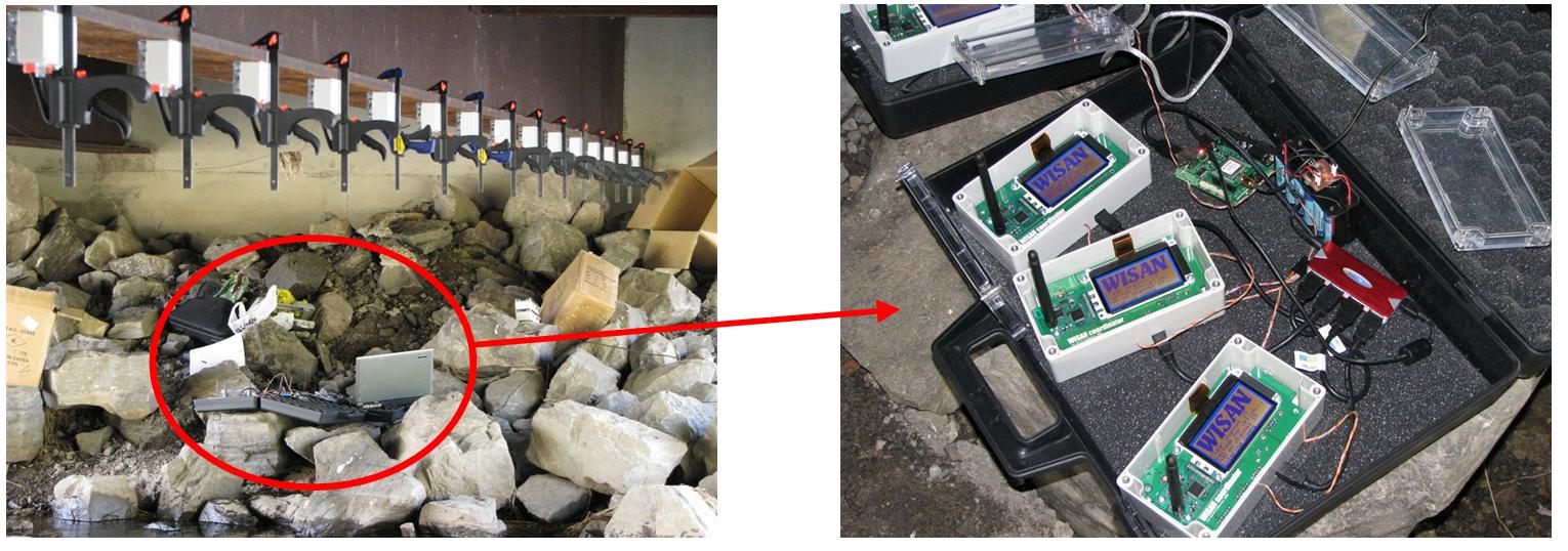
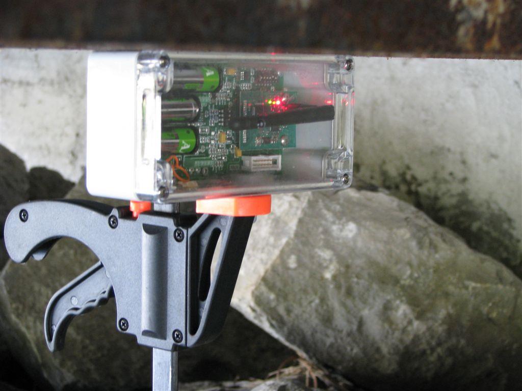
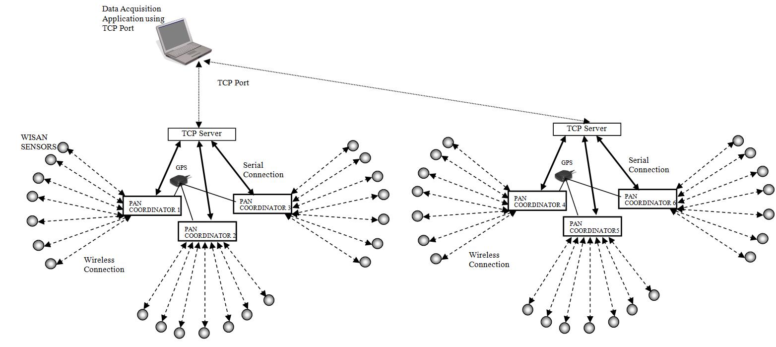
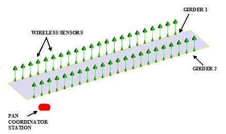
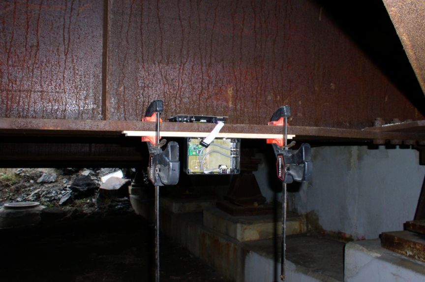
WISAN was originally designed to monitor structures built using steel girder technology. However, the same principles could be applied to modal testing of pre-stressed concrete structures. The presented experiment had the goal of demonstrating that reconstruction of mode shapes of a pre-stressed concrete bridge is possible from the data captured by a time-synchronized sensor network. The bridge on Route 1 at Kuala Lumpur, Malaysia was chosen as the test location (Figure 1). The bridge is built using 22 pre-stressed concrete girders with integral abutment. Total length of the bridge is 18m, width is 22m. The highest point is 5m above ground level with easy access to girders available in area of about 3m from both supports (Figure 2). Due to accessibility limitations the network was setup by attaching 22 sensors to 11 middle girders at a distance of 2.8m from both supports as shown in Figure 3. Thus, the dimension of the part of the structure that was tested is 18m x 10m. The sensors were clamped to the side of an aluminum plate glued to the girder as shown in Figure 4. The PAN Coordinator station is placed under the bridge on the bottom left of the entire setup. The PAN Coordinator station consisted of 3 PAN Coordinators connected to a laptop via serial interface. GPS was used to provide pulse per second synchronization signal to the PAN Coordinators. The network configuration for the test is as shown in Figure 5.

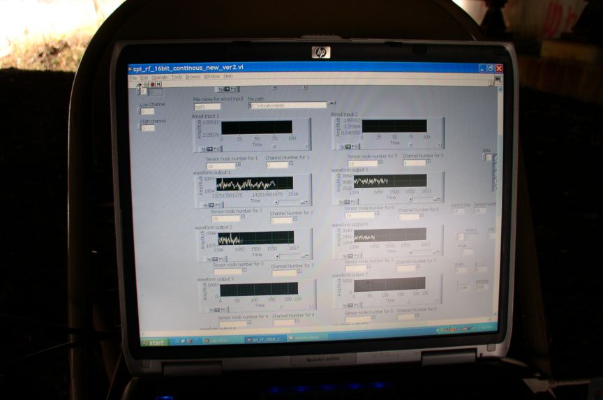
The sensors formed three network clusters on three independent frequency channels. Acceleration data was sampled at the rate of 240.385 Hz and a data resolution of 14 bits. The cut-off frequency of the programmable filter was set to 100 Hz. Vehicular traffic over the bridge was the source of excitation. Acceleration data from the sensors were recorded for time intervals of 2 minutes, 5 minutes and 10 minutes. The data collected from all the sensors was processed using the output-output modal analysis software ARTeMIS.

Results

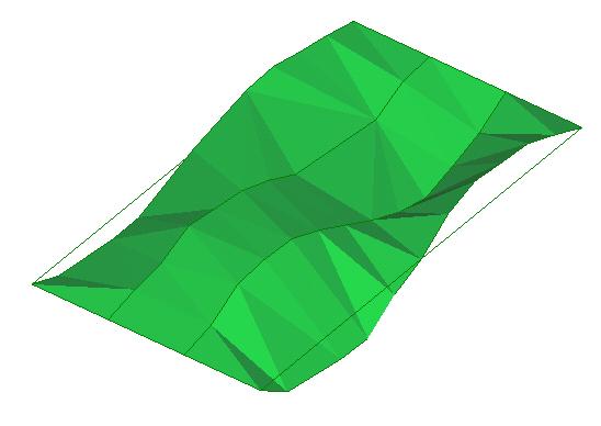
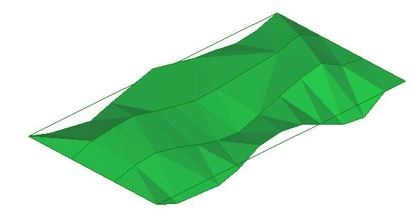
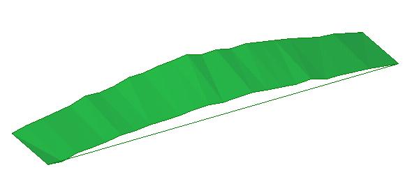
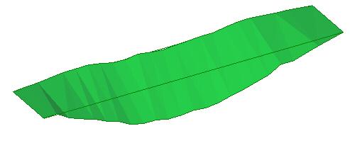
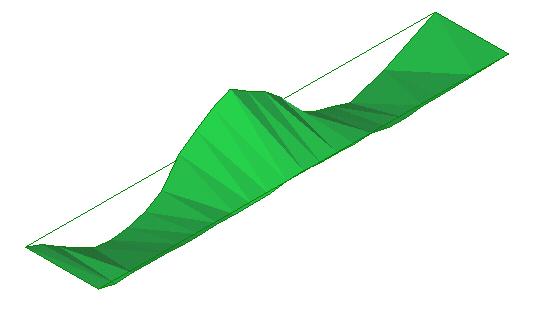
The acceleration response from each sensor location was processed using ARTeMIS and peaks were identified corresponding to the modal frequencies. Corresponding bending mode shapes have been plotted in Figure 8 – Figure 9 by using the relative sensor amplitude at a particular mode frequency.

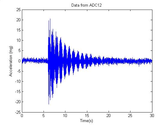
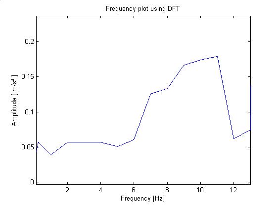
Acceleration data from a sensor located on the second girder (Figure 10) suggests a peak amplitude in the frequency spectrum of around 28 mg in the range of 8 – 12 Hz. Assuming this corresponds to the amplitude of the first bending mode observed at 10.74 Hz, the maximum displacement at the center (interpolating the data) would be around 50mg. With the sensor noise resolution of 0.5mg, the peak data resolution possible is around 7 bits out of 12 bits possible.

It is interesting to compare the results obtained from the concrete structure to those of a similarly-sized steel girder structure. In our previous work, we used WISAN to extract mode shapes from a RT31 steel bridge located in the Town of Lisbon, New York. This bridge has four steel girders (3m apart) and overall dimensions 19m x 10m. The bridge was equipped with 44 sensors, 11 sensors spaced equidistantly on each girder.

Comparison between the concrete and steel structures shows that both bridges have comparable modal frequencies predominantly in the range of 10Hz-30Hz. However, there is a significant difference in the maximal amplitude attained by the structural components. Testing of the concrete RT1 bridge in Kuala Lumpur was conducted under constant heavy traffic including heavy vehicles. The maximal amplitude of vibration at a distance of 2.8m from supports was 28 mg. Testing of the RT31 steel girder bridge in New York was under intermittent traffic with the most of one light vehicle on the bridge at a time. The maximal amplitude of vibration at a distance of 2.845m from supports was 24 mg. As these results show, a steel bridge achieved comparable levels of excitation under a much lighter traffic. Practically this means that vibration sensors with lower noise floor are necessary for monitoring of pre-stressed concrete structures since vibration levels may be lower than those of steel girder bridges.

Fig1a - RT1 bridge Fig1b - RT1 bridge

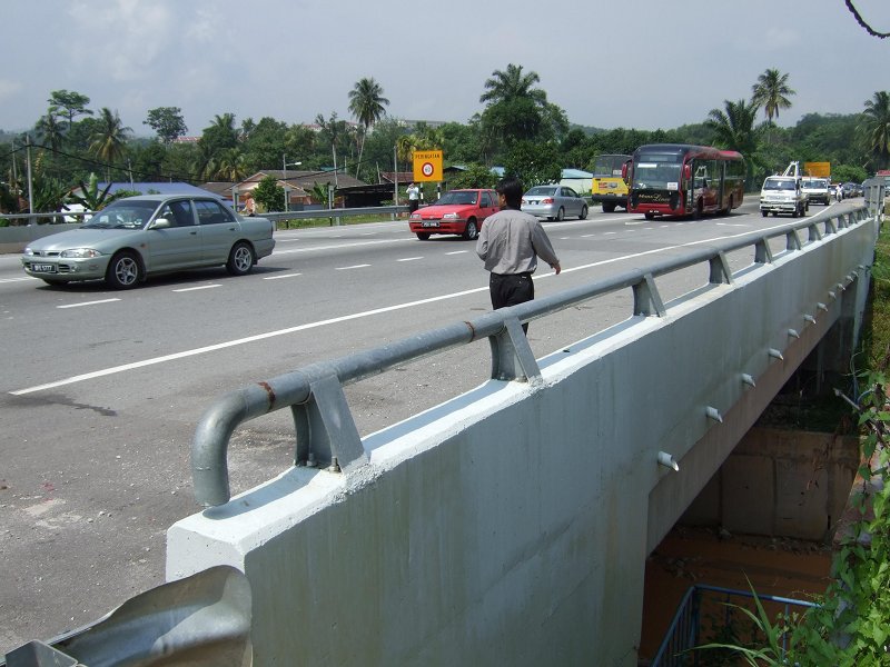
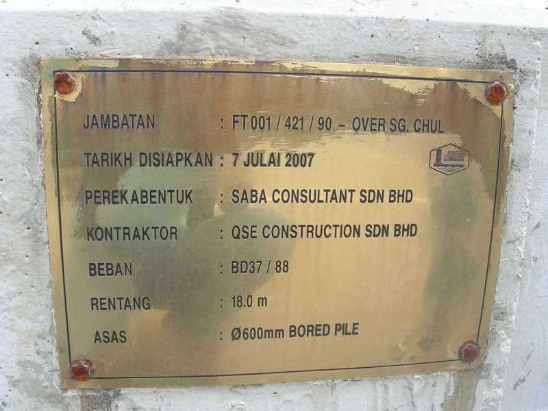
Figure 1 (a): Photo of the bridge on Route 1 and (b) details of the bridge from the test site

Fig2 - under the RT1 bridge

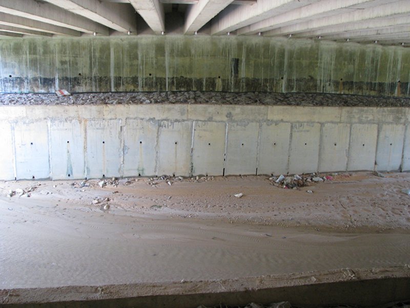
Figure 2: View from under the bridge

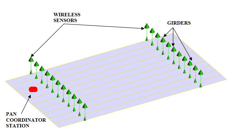
Fig3 - layout of wireless sensor network

Figure 3: Layout of the bridge test setup for the four girder grid setup

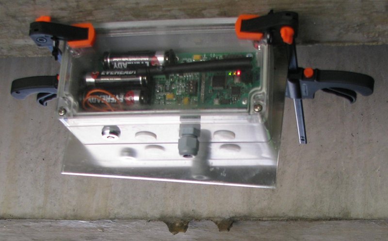
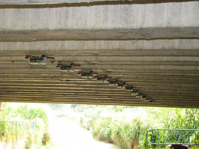
Fig4a - sensor attached to the bridge Fig4b - WISAN sensors on a bridge

Figure 4: View of (a) single sensor and (b) 11 sensors attached to the girders

Fig5 - network configuration

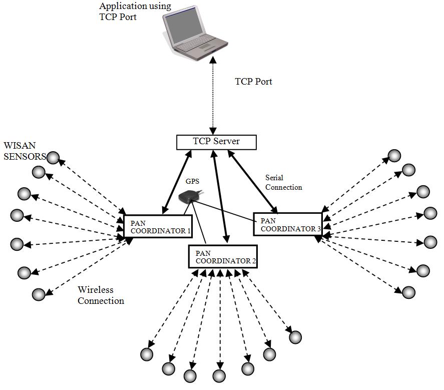
Figure 5: network configuration

Fig6 - mode shapes

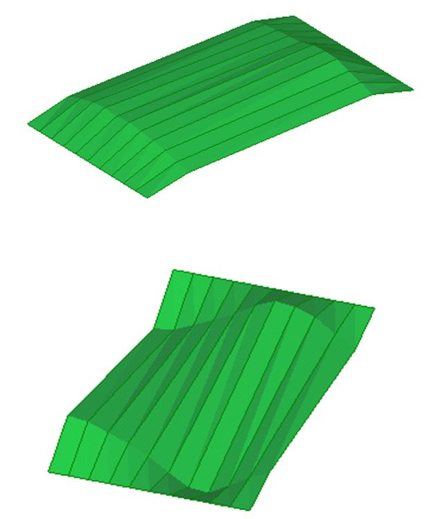
Figure 6: Mode shapes along the length of the bridge at frequencies (a) 10.74 Hz and (b) 32.1 Hz

Fig7 - higher mode shapes

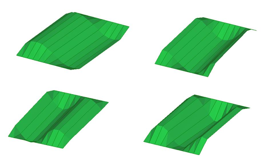
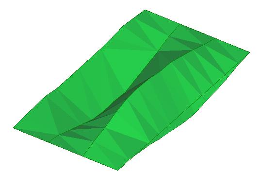
Figure 7: Mode shapes along the width of the bridge at frequencies (a)15.43Hz (b) 18.49 Hz (c) 23.18 and (b) 29.05 Hz

May 2008. WISAN testing on a bridge in New York state

WISAN testing on a bridge

The bridge (Figure 1(a)(b)) was tested in 2 setups using 44 sensors in on two girders and four girders respectively. The sensors were clamped on the bottom of the girders to provide a clear line-of-sight to the PAN Coordinator station (Figure 2) placed under the bridge on the bottom left of the entire setup. The PAN Coordinator station consisted of 6 PAN Coordinators connected to a laptop via serial interface. GPS was used to provide pulse per second synchronization signal to the PAN Coordinators. TCP based server was used to send / receive data from the network. LabView based client application was used to control the data collection process. The network configuration for the tests is shown in Figure 3.

The sensors formed six network clusters on six independent frequency channels that synchronized within ±23 µs using a synchronizing signal provided by the GPS receiver. Acceleration data was sampled at the rate of 240.385 Hz and a data resolution of 14 bits. Traffic passing over the bridge was the source of bridge excitation. Number of data recordings for the three setups were taken for 30 seconds, 2 minutes, 5 minutes and 10 minutes were taken. The cut of frequency of the programmable filter was varied between 100 Hz and 40 Hz to filter out high frequency noise components. Figure 4 shows a time series data for a sensor located near the center of the second girder. The frequency spectrum of the data shows peak amplitude of around 25 mg in the range of 8 – 12 Hz. This corresponds to roughly 6% of the total resolution of the ADC and which is approximately only 6 bits of sensor resolution which is much lower to that seen from the bridge on Route 11 in Potsdam.

7.27a 7.27b

(a) (b)

Figure 1: Different views of the bridge on Chipman Road

7.28a(1) 7.28a(3)

(a)

7.28b

(b)

7.28c

(c)

Figure 2: (a) Placement of WISAN sensors under the bridge (b) PAN Coordinator Station (c) Wireless Sensor clamped to the girder on the bridge

7.29

Figure 3: Network configuration for bridge testing (click to enlarge)

7.30a 7.30b

Figure 4: (a) Acceleration data from sensor located near the center of second girder. (b) Frequency spectrum of data from sensor located near the center of second girder.

Four Girder Grid Setup

In the first setup, all four girders were equipped with 11 sensors each. The layout of the test setup is shown in Figure 5.

7.31(0)

Figure 5: Layout of the bridge test setup for the four girder grid setup

The data collected from all the sensors was processed using the output-output modal analysis software ARTeMIS. Mode shapes from the four girder grid setup were successfully identified as summarized in Table 1 and shown in Figure 6 – Figure 10.

Mode Number	Frequency (Hz)
1	9.155
2	32.75
3	53.65

Table 1 (a): Vibration modal frequencies along the length of the bridge

Mode Number	Frequency (Hz)
1	10.97
2	26.23

Table 1 (b): Vibration modal frequencies along the width of the bridge

7.31(1) 7.31(2)

Figure 6: Three dimensional view of the first mode at 9.155 Hz obtained along the length of the bridge for four girder grid setup

7.32

Figure 7: Three dimensional view of the second mode at 32.75 Hz obtained from four girder grid setup

7.33

Figure 8: Three dimensional view of the third mode obtained at 53.65 Hz obtained from four girder grid setup

7.34(1) 7.34(2)

Figure 9: Three dimensional views of the first mode at 10.97 Hz obtained along the width of the bridge (side mode)

7.35

Figure 10: Three dimensional view of the second mode at 26.23 Hz obtained along the width of the bridge

Two girder grid setup

In the second setup, first two girders were equipped with 22 sensors each as shown in Figure 11. The mode shapes obtained are shown in Figure 12 to Figure 15.

7.36

Figure 11: Layout of the bridge test setup for the two girder grid setup

7.37 7.38

Figure 12: Three dimensional view of the 1^st longitudinal modes identified at 9.155 Hz using the two girder grid setup.

7.39

Figure 13: Three dimensional view of the 2^nd side modes identified at 26.23 Hz using the two girder grid setup.

Nov. 2004. Field test of WISAN

Field test on RT11 bridge

This is the first field test of WISAN. The tasks for this test included:

Comparison of wired data transmission vs wireless transmission of WISAN
Preliminary testing of different acceleration sensors
Identification of natural frequencies, and range of accelerations and displacements from ambient excitation

Vibration data were acquired using a custom made sensor module that interfaced a MEMSIC MXR2999 and an Applied MEMS SF1500S acceleration sensors. The output of each sensor was buffered and connected to the 12-bit ADC of a WISAN node and to a 16-bit USB data acquisition system. Data acquisition software was written in Labview and supported simultaneous data acquisition from the wireless and wired interfaces at 100Hz sampling rate.

The following figures show the sensor module and Labview interface.

sensor_box labview_interface

Two sensor modules were placed on the overpass bridge over Raquette river on RT11 in Potsdam, NY. The temperature during the test was about 32F or 0C. The bridge was excited by passing traffic.

Both sensors were attached on the girder number 4 under the deck. One of the sensor boxes was attached in the close proximity of the support column, while another sensor box was attached at various locations.

bridge_support_location Sensor location close to a support column.

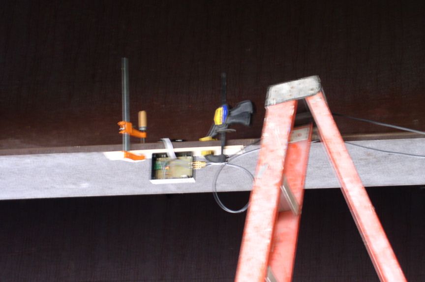bridge_midspan_sensor First sensor location. Midspan of the girder

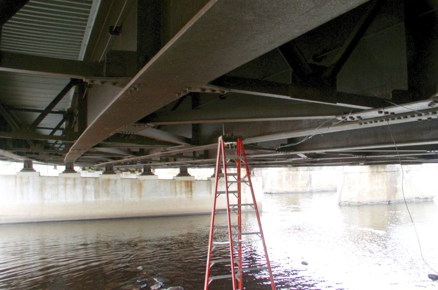bridge_midspan_location First sensor location. Midspan of the girder.

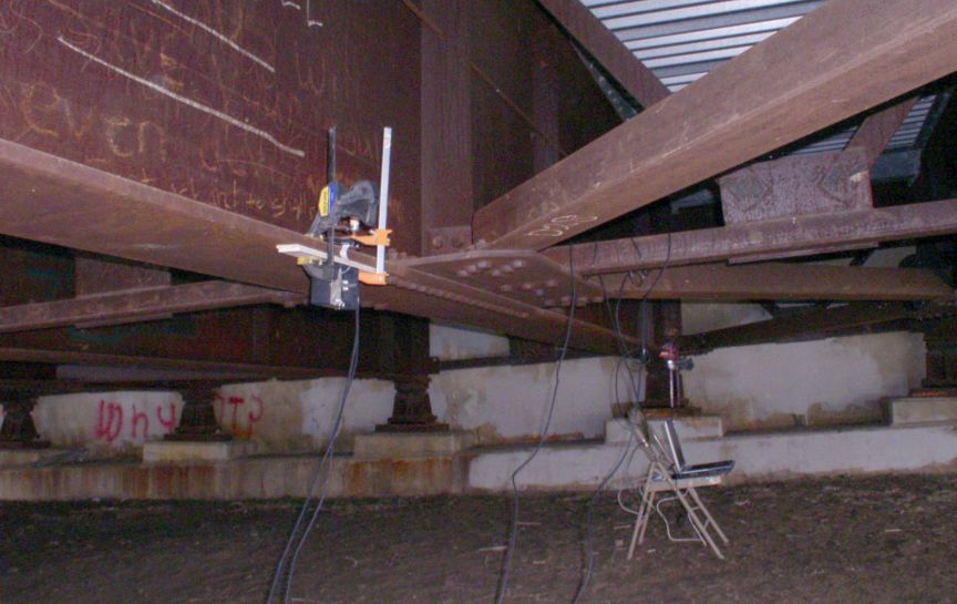sensor_at_location_2 Second sensor location: Moving closer to the support.

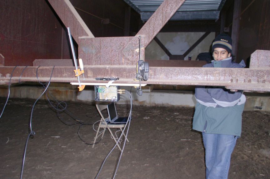sensor_at_location_3 Third sensor location

Some results

Test has shown very good correlation between wired and wireless data. The slight difference in results is caused by sample-to-sample asyncronization on the order of 10ms.

Wired data from Applied MEMS sensor (normalized by average)

Wireless data from the same sensor

Overplot of wireless and wired data shows good visual match between time series

Cross-correlation function of the time domain wired and wireless series clearly indicates a single point of the best match between series.

Power spectral density of the wired time series

Power spectral density of the wireless time series

Overplot of the frequency data indicates very good match in in the 10Hz frequency band.

The cross-correlation function in the frequency domain is almost identical to the cross-correlation function in time domain and indicates a single point of best match between the wired and wireless data